单变量线性回归——Pytorch实现

吴恩达老师机器学习课程中的线性回归采用的是Matlab编写的，我用Pytorch实现一遍。

x_train是房子大小

y_train是房子售价

最终目标是预测y_train

%matplotlib inline

使用numpy读入txt数据，np.loadtxt()

numpy.loadtxt(fname, dtype=<class 'float'>, comments='#', delimiter=None, converters=None, skiprows=0, usecols=None, unpack=False, ndmin=0, encoding='bytes')

从TXT文件中读入数据 文件中的每一行需要有相同的个数的数据

参数 fname : 文件名或者文件路径

dtype : 数据格式，可选，默认是float类型

comments : str or sequence of str, optional

The characters or list of characters used to indicate the start of a comment. None implies no comments. For backwards compatibility, byte strings will be decoded as ‘latin1’. The default is ‘#’.

delimiter : str, optional

The string used to separate values. For backwards compatibility, byte strings will be decoded as ‘latin1’. The default is whitespace.

converters : dict, optional

A dictionary mapping column number to a function that will parse the column string into the desired value. E.g., if column 0 is a date string: converters = {0: datestr2num}. Converters can also be used to provide a default value for missing data (but see also genfromtxt): converters = {3: lambda s: float(s.strip() or 0)}. Default: None.

skiprows : int, optional

Skip the first skiprows lines; default: 0.

usecols : int类型或者sequence类型，可选

Which columns to read, with 0 being the first. For example, usecols = (1,4,5) will extract the 2nd, 5th and 6th columns. The default, None, results in all columns being read.
Changed in version 1.11.0: When a single column has to be read it is possible to use an integer instead of a tuple. E.g usecols = 3 reads the fourth column the same way as usecols = (3,) would.

unpack : bool, optional

If True, the returned array is transposed, so that arguments may be unpacked using x, y, z = loadtxt(...). When used with a structured data-type, arrays are returned for each field. Default is False.

ndmin : int类型，可选，返回的array里至少有ndmin大小的维度

encoding : str类型，可选，对输入的文件进行编码设置，默认是'bytes'

Returns:

out : ndarray

Data read from the text file.

导入数据

import numpy as np
x_train = np.loadtxt('ex1data1.txt', delimiter=',', usecols=0, dtype=np.float32)
y_train = np.loadtxt('ex1data1.txt', delimiter=',', usecols=1, dtype=np.float32)
#print(x_train)
#print(y_train)

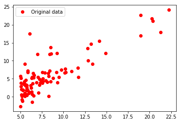
将数据用matplotlib画出来

import matplotlib.pyplot as plt
plt.plot(x_train, y_train, 'ro', label='Original data')
plt.legend()
plt.show()

png

设计并训练模型

import torch
import torch.nn as nn
import numpy as np
import matplotlib.pyplot as plt

input_size = 1
output_size = 1
num_epochs = 1000
learning_rate = 0.001

#dataset
x_train = np.loadtxt('ex1data1.txt', delimiter=',', usecols=0, dtype=np.float32).reshape((97,1))
y_train = np.loadtxt('ex1data1.txt', delimiter=',', usecols=1, dtype=np.float32).reshape((97,1))

#Linear regression model
model = nn.Linear(input_size, output_size)


#Loss and optimizer
criterion = nn.MSELoss()
optimizer = torch.optim.SGD(model.parameters(),lr=learning_rate)

#Train and model
for epoch in range(num_epochs):
    inputs = torch.from_numpy(x_train)
    targets = torch.from_numpy(y_train)
    #Forward pass
    outputs = model(inputs)
    loss = criterion(outputs, targets)
    #Backward and optimize
    optimizer.zero_grad()
    loss.backward()
    optimizer.step()
    if (epoch+1)%100 == 0:
        print('Epoch [{}/{}],Loss:{:.4f}'.format(epoch+1, num_epochs, loss.item()))
   
#plot the graph
predicted = model(torch.from_numpy(x_train)).detach().numpy()
plt.plot(x_train, y_train, 'ro', label='Original data')
plt.plot(x_train, predicted, label='Fitted line')
plt.legend()
plt.show()

Epoch [100/1000],Loss:11.1643
Epoch [200/1000],Loss:11.0105
Epoch [300/1000],Loss:10.8674
Epoch [400/1000],Loss:10.7343
Epoch [500/1000],Loss:10.6104
Epoch [600/1000],Loss:10.4951
Epoch [700/1000],Loss:10.3879
Epoch [800/1000],Loss:10.2881
Epoch [900/1000],Loss:10.1953
Epoch [1000/1000],Loss:10.1089

png